20. September 2024 By Immo Weber and Sascha Windisch
GraphRAG: Utilising complex data relationships for more efficient LLM queries
Anyone who has ever observed a squirrel in the forest may have noticed that it buries acorns in various places in the ground. Although the food is intended as a supply for the winter, the animals often forget their food stores. The forest is large and finding each acorn could take a long time.
Imagine if the squirrel had a detailed map showing not only where the acorns are buried, but also how these different hiding places are connected. With this map, you can go to the places where the most valuable acorns are buried without wandering around the forest without a plan.
Similar to the squirrel searching for its supplies, companies and authorities are often faced with the challenge of finding relevant information in huge amounts of data. Although Retrieval Augmented Generation ( RAG ) is still a relatively new technology for targeted retrieval of local domain knowledge, the technology often fails to aggregate complex distributed information. This is where GraphRAG comes into play.
Classic Retrieval Augmented Generation
GraphRAG is a synthesis of RAG and ‘knowledge graphs’. We have already covered the topic of RAG in detail in previous blog post, so we will only briefly summarise it here. RAG is a technique or system architecture for enriching the context of language models (Large Language Models, LLM) such as GPT-4o (OpenAI) with specific knowledge. This additional knowledge can include highly specific local domain knowledge that was not part of the training data of the LLM. The great advantage of RAG is that this knowledge can be provided and queried dynamically without the need for time-consuming and costly fine-tuning or retraining.
The use of RAG is divided into a preparation phase and an inference phase. In the preparation phase, source documents are prepared, segmented into text blocks (chunks), converted into a numerical format (vectors) using an embedding model and finally stored in a vector database. If the user sends a query to the RAG system during the inference phase, it is first vectorised and then a similarity search is carried out. This searches for the text segments in the vector database that are most similar to the original query. The most similar segments are then passed to a language model together with the query in order to generate the final response.
Where classic RAG reaches its limits
The classic RAG architecture works well when queries can be answered using explicit information from the source documents. Ideally, the answer to a query can be found directly in a stored source document. However, if an answer requires a combination of information from different source documents, the classic RAG architecture quickly reaches its limits.
This is due in particular to the way in which classic RAG finds relevant text segments from the source documents that match a query (‘retrieval’ phase). Traditionally, a semantic similarity search is performed within the stored source documents. However, this does not lead to a clear result if the relevant information is distributed across several documents or if the information searched for is only indirectly related to each other.
An example of such a query could be: ‘How has climate policy influenced global CO2 emissions in the last two decades?’ This query requires a combination of information from different time periods and documents, which may cause the RAG architecture to struggle to provide a precise answer. In such cases, the semantic similarity search can identify individual relevant segments, but the classic RAG architecture often fails to combine these segments in a way that produces a coherent and precise answer. This leads to a loss of information or inaccurate answers, as the retrieval phase is not designed to recognise and link complex relationships between different documents.
To answer more complex queries, there are a variety of advanced RAG techniques that are continuously being developed. Possible approaches include ‘query transformation’ or ‘context enrichment’ (see blog post From RAGs to Riches). A new technique is the synthesis of classic RAG and the concept of so-called knowledge graphs, which can initially be traced back to the paper G-Retriever: Retrieval-Augmented Generation for Textual Graph Understanding and Question Answering by He et al. (2024).
What are knowledge graphs?
Before we look at the topic of GraphRAG in more detail, we would like to give a brief overview of knowledge graphs. A knowledge graph is a data-driven structure that represents knowledge in the form of entities (people, places, objects) and the relationships between these entities. In contrast to traditional databases, which often store information in isolated tables, a knowledge graph links data in a way that makes it possible to recognise and analyse complex relationships and interactions between different points of information.
A knowledge graph consists of three main components:
- Entities (nodes): These represent the basic units of information, such as ‘Berlin’ as a city, ‘Benoit Mandelbrot’ as a person or ‘Artificial Intelligence’ as a concept.
- Relationships (edges): These describe the connections between entities. For example, the relationship between ‘Benoit Mandelbrot’ and ‘fractal geometry’ could be represented as ‘developed’, or the relationship between ‘Berlin’ and ‘Germany’ as ‘capital of’.
- Attributes (properties): These provide additional information about the entities or relationships. For example, an entity ‘Albert Einstein’ could have attributes such as ‘Year of birth: 1924’ or ‘Nationality: French’.
The main advantage of a knowledge graph lies in its ability to capture contextual information and thus enable a deeper understanding of the data. For example, if a search query is made for ‘famous mathematicians’, a knowledge graph can provide not only a list of mathematicians, but also relevant information about their works, areas of influence and connections to other scientists.
From RAG and graphs to GraphRAG
Having looked at both classic RAG and knowledge graphs individually, the legitimate question now arises as to how these two techniques can be meaningfully combined. In fact, two complementary approaches are conceivable, which can be roughly reduced to two processes:
- 1. indexing
- 2. querying
Indexing: Creating knowledge graphs using LLM
The process of indexing, i.e. the creation of knowledge graphs using LLM, can also be used independently of integration into GraphRAG. In the context of GraphRAG, however, this process essentially corresponds to the preparation phase in classic RAG systems (see blog post Retrieval Augmented Generation). However, instead of a (pure) vector database, a so-called (hybrid) graph database can be used to store the data.
As with classic RAG, the process begins
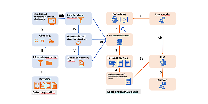
- I) with the extraction and
- II) the segmentation of text blocks (Figure 1). As with classic RAG, advanced segmentation methods such as context expansion can theoretically also be used here (see blog post From RAGs to Riches). However, instead of vectorising the text segments directly using the embedding model, we first
- IIIa) entities and relationships are extracted from these using a language model. In addition, similar to the HyDe (‘Hypothetical Document Embedding’) approach (see blog post From RAGs to Riches)
- IIIb), the core statements of the respective text segments can be linked to the entities and relationships. Using the Leiden method, the next step is to
- IV) the extracted entities and their relationships are clustered into communities. A community is a local network of densely connected nodes that have only a few connections to other communities. In the final indexing step
- V) hierarchical summaries are created at community level. These community reports contain information about the most frequently contained entities, their connections and HyDe content. The knowledge graphs, vectorised entities and community reports created are finally
- VI) either separately or in a hybrid vector/graph database.

Figure 1: Indexing and query phase of a local GraphRAG enquiry. Left: Data preparation. Right: Query.
Queries: Using knowledge graphs to answer complex queries
In the query phase, a GraphRAG system can be used in two ways:
- 1) Querying global information
- 2) Querying local information.
Getting an overview: the macroscopic view
Global queries tend to ask more general questions of the data, which make it necessary to aggregate information at a macroscopic level. For example, one question could be: ‘What are the main contents of the data set?’ Community reports at higher hierarchy levels are primarily used for this purpose.
The procedure is as follows: Firstly, the community reports are combined in random batches and segmented again. Then each text segment is passed to an LLM together with the initial enquiry in order to generate an intermediate response. This intermediate response contains a list of points that are rated according to relevance. The most relevant points of all intermediate answers are finally passed to an LLM as context with the initial question to generate the final answer.
Under the magnifying glass: the microscopic view
Local queries are used to address more specific queries to your own data. The procedure here initially corresponds to the classic RAG process: The enquiry is first
- 1) vectorised using an embedding model (Figure 1). Then
- 2) a similarity search is carried out using the vectorised entities in order to
- 3) find the most relevant content. Starting from the knowledge graph
- 4) the closest relationships, neighbouring entities and associated community reports are extracted. The mapping of the vectorised entities to the knowledge graph can be done either via two separate databases (vector and graph database) or a single hybrid database. Finally, this content is stored as context
- (5a) together with the initial query
- (5b) to an LLM and
- (6) the final response is generated.
Advantages and disadvantages of GraphRAG
Similar to classic RAG, GraphRAG is not always the most efficient solution. Accordingly, depending on the use case, it should be weighed up whether the cost of an implementation is justified. In principle, the following advantages and disadvantages result from the approach.
Advantages of GraphRAG
- Explainability: The use of structured knowledge graphs offers a transparent and comprehensible representation of information, which strengthens confidence in the results and creates the basis for further analyses.
- Multi-layered analyses: GraphRAG is able to process complex queries from multiple perspectives by bringing together relevant information from different areas of the knowledge graph.
- More contextualised queries: Thanks to the knowledge graph, GraphRAG can understand the semantic connections and relationships between different concepts, leading to more precise and relevant results.
Possible disadvantages of GraphRAG
- Scalability challenges: As the complexity and size of the knowledge graph increases, so do the demands on computing power, which can be particularly problematic for real-time applications.
- Dependency on the underlying data: The effectiveness of GraphRAG depends heavily on the quality and completeness of the data sources used. If these are incomplete or distorted, this can impair the performance of the system.
- Complexity in building the knowledge graph: Creating an accurate and comprehensive knowledge graph requires careful prompt engineering to extract entities and model relationships, which can be time-consuming and technically challenging.
Code example for indexing and local GraphRAG query
We will again keep the coding example relatively simple, similar to the previous articles. It assumes a Python environment in which basic libraries have been installed. As usual, we will use the LlamaIndex library to encapsulate the AI calculations and calls.
LlamaIndex offers various connections to graph databases, of which we will use the graph database Neo4j in this example. This has the advantages that the database can be operated locally as an open source solution or in a Docker container and that we can display the content graphically.
The connection is made by creating a configuration for accessing the database.
		graph_store = Neo4jPropertyGraphStore(
		    username=‘***’,
		    password=‘***’,
		    url=‘bolt://localhost:7687’,
		    database=‘neo4j’,
		)
In the next step, we create the indexing object, to which we add the Neo4J connection and the language models to be used. A distinction is made between an LLM for creating the embedding vectors and an LLM for the subsequent text or response generation. In our example, we use the LLMs from OpenAI for both processes. However, other, local language models could also be used here. Here we specify the concrete language model and a temperature of 0, with which we indicate that the most relevant response is generated and that creativity, along with the risk of hallucinations, is rather negligible.
		index = PropertyGraphIndex.from_documents(
		    documents,
		    embed_model=OpenAIEmbedding(model_name=‘text-embedding-3-small’),
		    kg_extractors=[
		        SchemaLLMPathExtractor(
		            llm=OpenAI(model=‘gpt-3.5-turbo’, temperature=0.0)
		        )
		    ],
		    property_graph_store=graph_store,
		    show_progress=True,
		)
We also provide the graph extractor SchemaLLMPathExtractor as a parameter. This object can be used to set detailed parameters for the nodes and relationships of the graph so that a suitable graph can be created. In our example, we use the default values.
When the code is executed, the graph is created in Neo4j. With logging switched on, we can also see how the individual chunks from the document decomposition are sent to the LLM to create the embedding vectors.
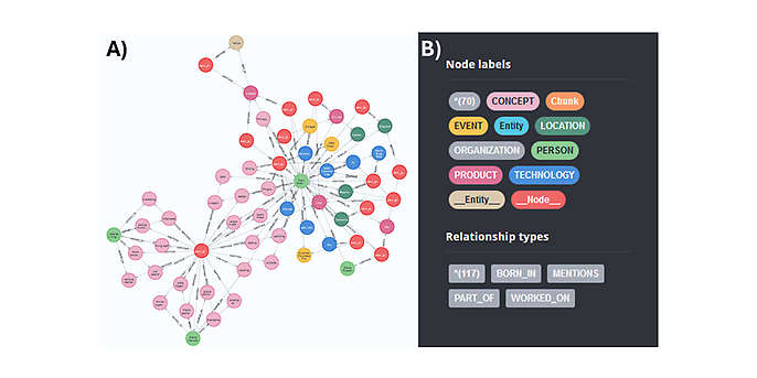
If we now look at the knowledge graph from a distance, we see the following picture of different relationships between the nodes. In our example, there appear to be two main nodes from which the graph has developed.

Figure 2: Database graph after the indexing phase. A) Visualisation of the graph) B) Properties, nodes and relationships.
Even without detailed configuration of the extractor, we can see in Figure 2B that the index has already created suitable labels for the nodes and relationship types.
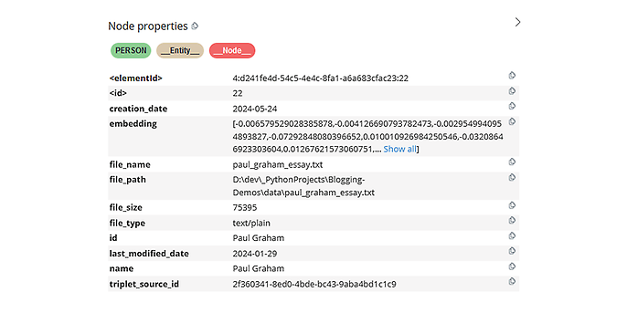
If we now take a closer look at the data of a node, for example ‘Paul Graham’, we not only see the source from which this node originated (file name), but also the embedding vector for this node, which can be used in the subsequent search.

Figure 3: Example metadata of a node.
Once generated, the database can be reused without having to create it again. To do this, we again create an index object, but this time based on the existing database.
		index = PropertyGraphIndex.from_existing(
		    property_graph_store=graph_store,
		    llm=OpenAI(model=‘gpt-3.5-turbo’, temperature=0.3),
		    embed_model=OpenAIEmbedding(model_name=‘text-embedding-3-small’),
		)
Once created, the graph can now be used for inferences (queries). To do this, a parameterisable query object (query engine) is first created.
		query_engine = index.as_query_engine(
		   include_text=True
		)
With the following query to the query engine, we receive a response object with the answer from the GraphRAG and the language model. In the response object, we recognise that several nodes were found and used for generation.
		response = query_engine.query(‘What happened at Interleaf and Viaweb?’)
		print(str(response))
We ask the compound question: 'What happened at Interleaf and Viaweb?’ and receive a longer complex answer: ‘Interleaf was one of many companies that had smart people and built impressive technology, but got crushed by Moore's Law. Viaweb, on the other hand, was a company that Paul Graham worked on, which allowed users to define their own page styles by editing Lisp expressions underneath.’
Summary and outlook
In this blog post, we presented the GraphRAG technology, which combines the advantages of classic retrieval augmented generation and knowledge graphs. LLM can be used to create knowledge graphs and graphs can also be used to answer complex RAG queries. The approach shows once again how versatile RAG technology can be used and what potential it still harbours. We will look at another approach to using RAG in connection with databases in the next article, in which we present Text2SQL, a technique for translating natural language queries into SQL syntax.
Would you like to find out more about exciting topics from the world of adesso? Then take a look at our previous blog posts.
Also interesting:


